


Infraschall - Messung und Auswertung
Ansprechperson: Dr. Stefan Holzheu
Powerspectraldensity (PSD) vs. Powerspektrum (PS)
Bei der Darstellung von Infrschallsignalen im Frequenzbereich gibt es zwei Methoden:
- PSD == Leistungsdichtespektrum
- PS == Schallampltiude einer betrachteten Frequenz-Auflösung == absoluter Schalldruck
Das PS eignet sich gut, um harmonische Signalbestandteile in ihrer Amplitude zu quantifizieren. Die PSD dagegen ist besser für zufällige Signale und zur Bewertung des allgemeinen Hintergrunds. Die Verfahren lassen sich auch ineinander umrechnen. Dies zeigt die folgende Grafik:
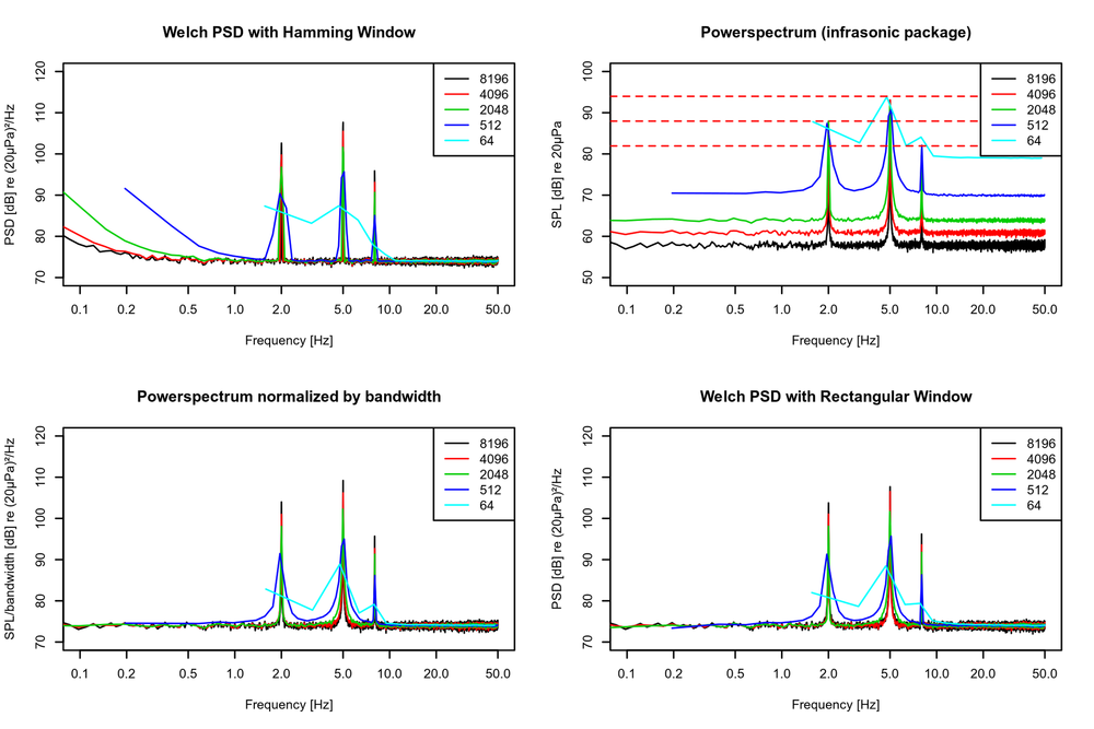 Plot 1 (links oben) ist eine PSD-Analyse mit Standard Hamming Window mit unterschiedlicher Länge. Plot 2 (rechts oben) ist die FFT Analyse, die mein R-Paket liefert. Man erkennt, dass das Rauschniveau von der Fensterlänge abhängt. Die Lage der Maximal ist jedoch für alle Auflösungen gleich und trifft sehr gut die theoretischen Werte (gestrichelte horizontale Linien).
Im Plot 3 (links unten) wurde die FFT über die Bandbreite normiert. Dies entspricht sehr genau einer PSD mit Rechteckfenster (oder auch "ohne" Fenster - siehe Plot 4 - rechts unten).
Hier das R-Skript, mit dem die Plots erzeugt werden:
## Length of dateset
l=5e5
# normal distributed noise
noise=rnorm(l)
# time-vector
t=(1:l)/100
# signal composed by three sinus
s=0.5*sqrt(2)*sin(2*pi*t*2)+1.0*sqrt(2)*sin(2*pi*t*5)+0.25*sqrt(2)*sin(2*pi*8*t)
# add noise + signal
v=noise+s

library(oce)
# create ts-Object with sampling frequency 100
xts=ts(v/20e-6,frequency = 100)

## Start Plot
par(mfrow=c(2,2))
par(cex=0.5)

############################################
#Plot1: Calculate and Plot PSD with Standard Hamming Window
ps2048=pwelch(xts,nfft=2048,plot=F)
ps4096=pwelch(xts,nfft=4096,plot=F)
ps8192=pwelch(xts,nfft=8192,plot=F)
ps512=pwelch(xts,nfft =512,plot=F)
ps64=pwelch(xts,nfft =64,plot=F)

plot(ps8192$freq,10*log10(ps8192$spec),type='l',log='x',
     xlim=c(0.1,50),ylab='PSD [dB] re (20µPa)²/Hz',xlab='Frequency [Hz]',main='Welch PSD with Hamming Window',ylim=c(70,120))
lines(ps4096$freq,10*log10(ps4096$spec),col=2)
lines(ps2048$freq,10*log10(ps2048$spec),col=3)
lines(ps512$freq,10*log10(ps512$spec),col=4)
lines(ps64$freq,10*log10(ps64$spec),col=5)
legend('topright',c('8196','4096','2048','512','64'),lty=1,col=1:5)

############################################
#Plot 2: Calculate and Plot FFT
d=data.frame(t,v)
library(infrasonic)
fft8192=infrasonic.calcFFT(d,res=100/8196,detrend = FALSE)
fft4096=infrasonic.calcFFT(d,res=100/4096,detrend = FALSE)
fft2048=infrasonic.calcFFT(d,res=100/2048,detrend = FALSE)
fft512=infrasonic.calcFFT(d,res=100/512,detrend = FALSE)
fft64=infrasonic.calcFFT(d,res=100/64,detrend = FALSE)

plot(fft8192$freq,fft8192$db,log='x',xlim=c(0.1,50),ylab='SPL [dB] re 20µPa',
     xlab='Frequency [Hz]',type='l',main='Powerspectrum (infrasonic package)',ylim=c(50,100))
lines(fft4096$freq,fft4096$db,col=2)
lines(fft2048$freq,fft2048$db,col=3)
lines(fft512$freq,fft512$db,col=4)
lines(fft64$freq,fft64$db,col=5)
abline(h=20*log10(0.5/20e-6),lty=2,col=2)
abline(h=20*log10(1/20e-6),lty=2,col=2)
abline(h=20*log10(0.25/20e-6),lty=2,col=2)
legend('topright',c('8196','4096','2048','512','64'),lty=1,col=1:5)

###########################################
#Plot3: Rescale Plot2 to PSD
fft2ps<-function(x,bw){
  p=20e-6*10^(x/20) #RMS Amplitude
  10*log10((p/20e-6)^2/2/bw) #psd
}
plot(fft8192$freq,fft2ps(fft8192$db,100/8196),log='x',
     xlim=c(0.1,50),ylab='SPL/bandwidth [dB] re (20µPa)²/Hz',
     xlab='Frequency [Hz]',type='l',main='Powerspectrum normalized by bandwidth',ylim=c(70,120))
lines(fft4096$freq,fft2ps(fft4096$db,100/4096),col=2)
lines(fft2048$freq,fft2ps(fft2048$db,100/2048),col=3)
lines(fft512$freq,fft2ps(fft512$db,100/512),col=4)
lines(fft64$freq,fft2ps(fft64$db,100/64),col=5)
legend('topright',c('8196','4096','2048','512','64'),lty=1,col=1:5)

############################################
#Plot4: Calculate and Plot PSD with rectangular Window
psr2048=pwelch(xts,window = rep(1,2048),plot=F)
psr4096=pwelch(xts,window = rep(1,4096),plot=F)
psr8192=pwelch(xts,window = rep(1,8192),plot=F)
psr512=pwelch(xts,window = rep(1,512),plot=F)
psr64=pwelch(xts,window = rep(1,64),plot=F)

plot(psr8192$freq,10*log10(psr8192$spec),type='l',log='x',
     xlim=c(0.1,50),ylab='PSD [dB] re (20µPa)²/Hz',xlab='Frequency [Hz]',main='Welch PSD with Rectangular Window',ylim=c(70,120))
lines(psr4096$freq,10*log10(psr4096$spec),col=2)
lines(psr2048$freq,10*log10(psr2048$spec),col=3)
lines(psr512$freq,10*log10(psr512$spec),col=4)
lines(psr64$freq,10*log10(psr64$spec),col=5)
legend('topright',c('8196','4096','2048','512','64'),lty=1,col=1:5)